2DGS-Planner

Planning directly on a 2DGS map of an outdoor courtyard. Left: Gaussian disks, the roadmap, and the planned path. Right: the rendered scene along the same path.

Abstract

Gaussian splatting provides an explicit and efficiently rasterizable scene representation for robot navigation. However, individual Gaussian primitives may not reliably represent obstacles as they are jointly optimized through alpha-composited rendering from a finite set of reconstruction views. We propose 2DGS-Planner, a path planner for ground robots that reads planning-relevant geometry from a 2D Gaussian splatting (2DGS) map through rasterization, rather than treating individual Gaussian primitives as obstacles. During offline roadmap construction, multi-view attribution converts rendered normal dispersion into structural scores for non-ground disks supported by the reconstruction views. These scores guide adaptive node sampling on the ground. Path-aligned orthographic queries validate candidate edges, while cylindrical queries estimate local clearance fields that are cached on the edges. During online planning, graph search initializes a route, and path refinement reuses the cached fields while accounting for the robot’s dimensions and ground constraints. Experiments demonstrate improved roadmap connectivity, more accurate clearance estimation, and higher planning success compared with the tested baselines. These results support rasterization as an effective geometric query interface for planning directly on Gaussian maps.

Planning results

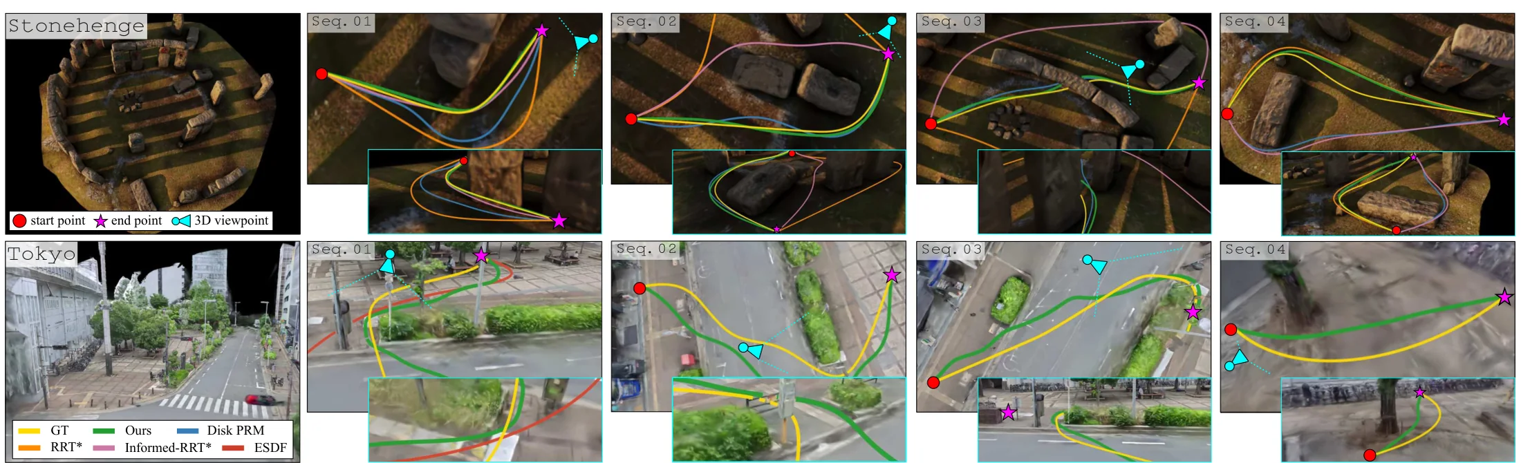
Paths from each planner for the same start–goal pairs, drawn in the 2DGS map.

Stonehenge

SPL 0.956 · 48/50 pass collision check

GT
Ours
Disk PRM
RRT*
Informed-RRT*
ESDF

Tokyo

SPL 0.782 · 40/50 pass collision check

GT
Ours
ESDF
Other methods failed to generate feasible paths.

Top-down view

Start–goal pairs 0–9 in each scene

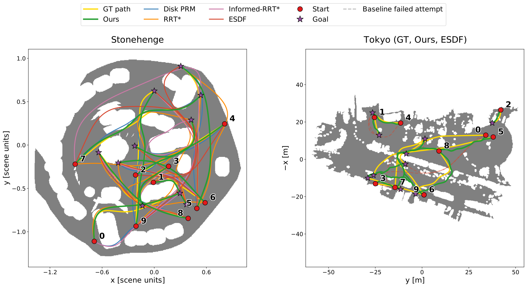
Top-down maps of Stonehenge and Tokyo with the paths of each method for start-goal pairs 0 to 9, drawn over the traversable ground. — Paths are B-spline-smoothed for display, as in the videos above. Tokyo shows GT, Ours, and ESDF; dashed lines are failed attempts. Click the map to zoom.

Our full planner (adaptive + refinement). SPL and collision-check counts at ε_ref over 50 start–goal pairs per scene. Full comparison in Results.

Real-world deployment

We plan a route in the 2DGS map of an indoor room, register the map to a FAST-LIO2 LiDAR map, and track the refined path on a humanoid robot with a pure-pursuit controller.

Left: planned path and robot body in the 2DGS map. Right: the humanoid robot executing the route. Insets show the rendered and real point of view. Played at 1.3× speed.

Why query the rendered surface?

Three views compare an RGB rendering, the individual Gaussian disks, and disks whose depths deviate from the composited surface. — (a) Rendered appearance. (b) The underlying 2D Gaussian disks. (c) Disks whose depth deviates strongly from the composited surface, shown in red. The rendering looks correct, but individual primitives are not reliable obstacles. 2DGS-Planner therefore queries the composited surface through rasterization instead.

Method

The full pipeline: preprocessing and multi-view attribution lead to adaptive sampling, orthographic edge screening, and cylindrical clearance caching; online A-star search and B-spline refinement produce the path and robot body poses. — **Overview.** Offline, we score surface structure from multiple views, sample ground nodes adaptively, screen edges with orthographic queries, and cache a cylindrical clearance field on each edge. Online, A* finds an initial route, which is refined as a B-spline using the cached clearance and then revalidated.

Rendered layers

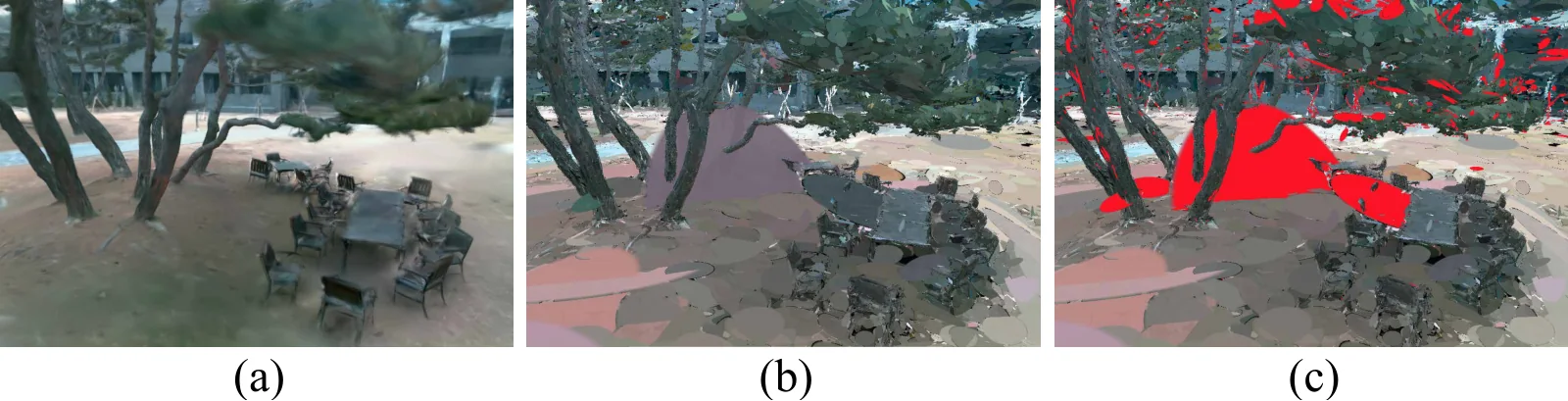
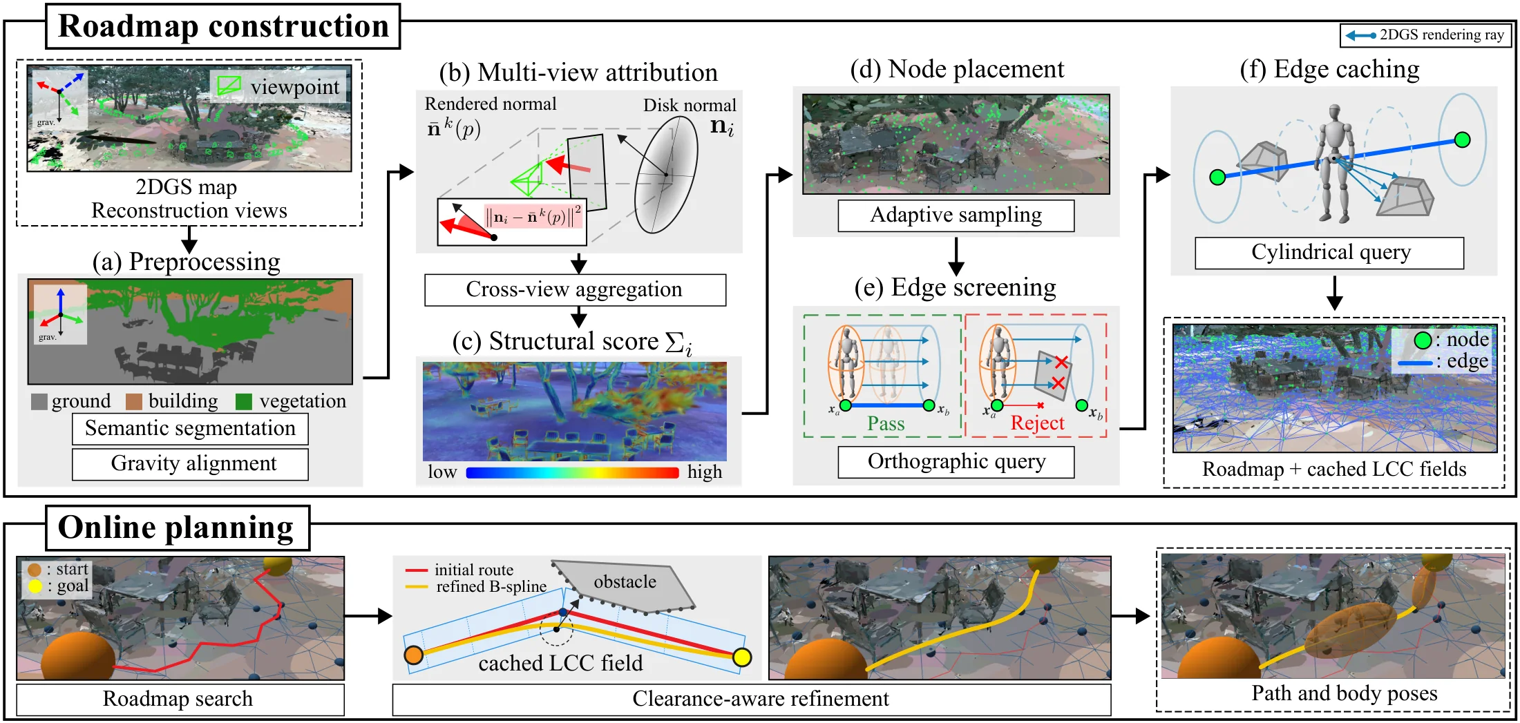
Everything the planner uses is read from rasterized views of the same map.

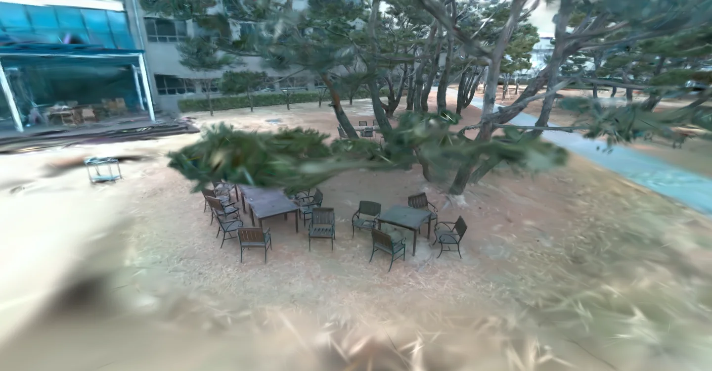
RGB rendering of the reconstructed outdoor courtyard with trees, chairs, and surrounding buildings.

RGB rendering of the reconstructed courtyard.

Pipeline stages

Offline · Roadmap construction

Multi-view attribution

Rendered normals are compared with each disk’s normal across reconstruction views. Planar regions show low dispersion; corners show high dispersion.

Structural score

Dispersion aggregated over the views becomes a score for each observation-supported non-ground disk.

Adaptive sampling

Ground nodes are sampled more densely near high-score structure and connected into a roadmap.

Edge screening

A path-aligned orthographic query renders along each candidate edge with the robot’s footprint. Edges whose rays hit a surface are rejected.

Clearance caching

A cylindrical query renders the radial distance to surfaces around the edge. It is unrolled into a local clearance field and cached on the edge.

Online · Path planning

Path refinement

The A* route is refined as a B-spline using the cached clearance, the robot’s dimensions, and ground support, then revalidated.

Adaptive vs. uniform sampling

With the same sampling budget, adaptive sampling places more nodes near corners and clutter. Drag the divider to compare.

Uniform roadmap sampling with orange edges. — Matched views from Fig. 4 of the paper.

Adaptive roadmap sampling with blue edges, denser around the sidewalk obstacles. — Matched views from Fig. 4 of the paper.

Results

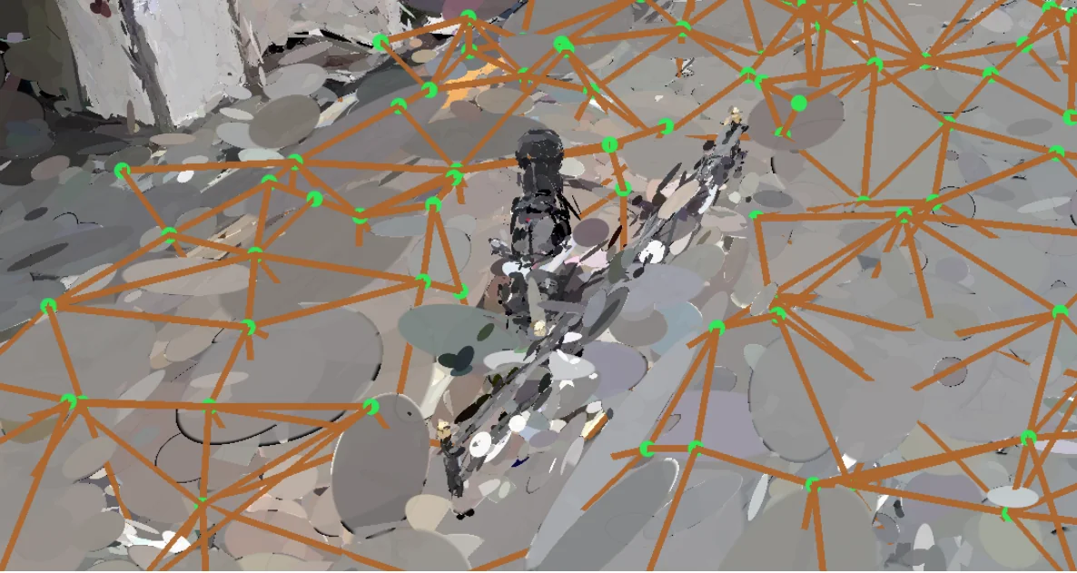
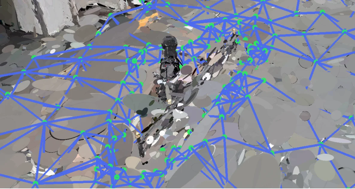
We evaluate 50 start–goal pairs in each of two scenes. All methods use the same 2DGS reconstruction. Stonehenge is synthetic and has an exact reference mesh (r = 0.05 scene units, ε_ref = 0.005). Tokyo is a real-world capture evaluated against an aligned proxy mesh (r = 0.50 m, ε_ref = 0.10 m).

Method	Stonehenge			Tokyo
Method	Pass (ε_ref)	Pass (ε = 0)	SPL	Pass (ε_ref)	Pass (ε = 0)	SPL
Disk PRM (1k)	21/50	15/50	0.335	6/50	6/50	0.091
Disk PRM (10k)	43/50	29/50	0.746	10/50	10/50	0.176
Disk PRM (60k)	45/50	27/50	0.810	10/50	9/50	0.168
RRT*	35/50	24/50	0.663	10/50	8/50	0.180
Informed RRT*	33/50	24/50	0.650	13/50	10/50	0.248
ESDF (ground-constr.)	38/50	26/50	0.751	12/50	8/50	0.218
Ours (uniform)	38/50	26/50	0.752	38/50	30/50	0.694
Ours (uniform) + refinement	40/50	31/50	0.781	39/50	33/50	0.717
Ours (adaptive)	46/50	31/50	0.917	40/50	32/50	0.765
Ours (adaptive) + refinement	48/50	34/50	0.956	40/50	34/50	0.782

Table I. Collision pass counts at ε_ref and at ε = 0, and SPL. Higher is better. Best values in bold.

Representative trajectories of each planning method for four start-goal pairs in Stonehenge and Tokyo. — Representative trajectories for four pairs in each scene. Colors identify the planning method.

Comparison of LCC and ESDF clearance error, false-safe and false-blocked rates, memory, and build time. — **Clearance fidelity** on 5,716 near-boundary queries. LCC and ESDF use the same rendered surface samples. LCC has lower clearance error and fewer false-blocked configurations, though false-safe cases remain.

Mean online planning latency per method for Stonehenge and Tokyo. — **Online latency**, averaged over 50 requests including failures. Refinement costs 0.357 s per request on Stonehenge and 1.11 s on Tokyo.

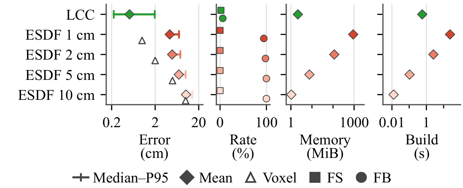
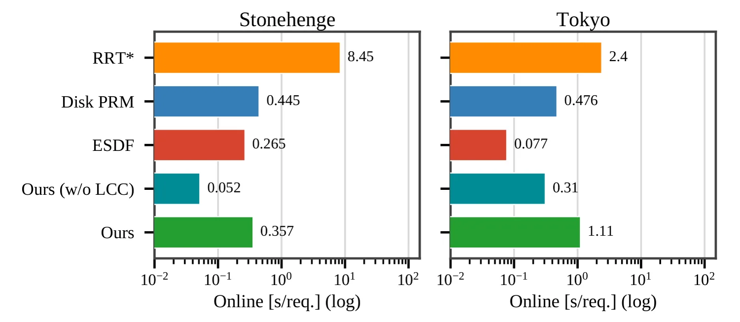
Hardware: RTX 4090, Core i9-10900K, 94 GB RAM. Each edge caches a 64 × 128 clearance field, and refinement uses 12 B-spline control points. Scope: fixed maps, an ellipsoidal robot body, and ground-supported paths.

Planning for the robot’s body

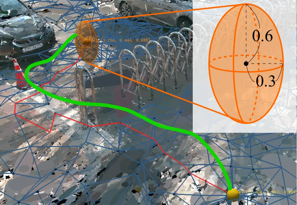
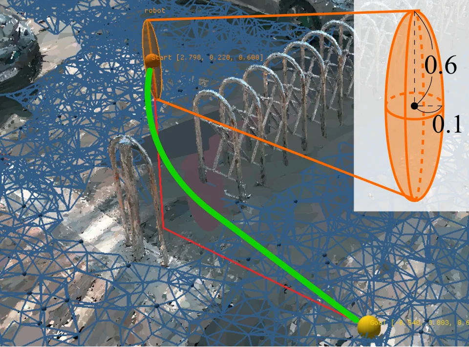
Footprint queries depend on the robot’s size, so the same start and goal can produce different routes.

With a lateral half-width of 0.3 m, the robot follows the wider passage around a railing. — Lateral half-width 0.3 m: the path takes the wider passage around the railing.

With a lateral half-width of 0.1 m, the robot takes the narrower passage for a shorter path. — Lateral half-width 0.1 m: the narrow gap is feasible, which gives a shorter path.

Robot body poses along a refined path.

Citation

BibTeX will be added once the paper is public.